Open Wake Word on the Web

How I Ported a Python Wake Word System to the Browser When the LLMs Gave Up

I started this project with a goal that seemed simple on paper: take openWakeWord, a powerful open-source library for wake word detection, and make it run entirely in a web browser. And when I say “in the browser,” I mean it. No tricks. No websockets streaming audio to a Python server. I wanted the models, the audio processing, and the detection logic running completely on the client.
My initial approach was to “vibe-code” it with the new generation of LLMs. I fed my high-level goal to Gemini 2.5 Pro, o4-mini-high, and Grok 4. They gave me a fantastic head start, building out the initial HTML, CSS, and JavaScript structure with impressive speed. But after dozens of messages just refining the vibe, we hit a hard wall. The models would run, but the output score was just a flat line at zero. No errors, no crashes, just… nothing.
This is where the real story begins. The vibe was off. Vibe coding had failed. I had to pivot from being a creative director to a deep-dive detective. It’s a tale of how I used a novel cross-examination technique with these same LLMs to solve a problem that each one, individually, had given up on.

TL;DR: The openWakeWord JavaScript Architecture That Actually Works

For the engineers who just want the final schematics, here is the stateful, multi-buffer pipeline required to make this work.

• Pipeline: [Audio Chunk] -> Melspectrogram Model -> Melspectrogram Buffer -> Embedding Model -> Wake Word Model -> Score
• Stage 1: Audio to Image (Melspectrogram):
  • Audio Source: 16kHz, 16-bit, Mono PCM audio.
  • Chunking: The pipeline operates on 1280 sample chunks (80ms). This is non-negotiable.
  • Model Input: The chunk is fed into melspectrogram.onnx as a float32 tensor.
  • Mandatory Transformation: The output from the melspectrogram model must be transformed with the formula output = (value / 10.0) + 2.0.
• Stage 2: Image Analysis (Feature Embedding):
  • Melspectrogram Buffer: The 5 transformed spectrogram frames from Stage 1 are pushed into a buffer.
  • Sliding Window: This stage only executes when the mel_buffer contains at least 76 frames. A window is sliced from the start of the buffer.
  • Model Input: This window is fed into embedding_model.onnx as a tensor.
  • Window Step: After processing, the buffer is slid forward by 8 frames (splice(0, 8)).
• Stage 3: Prediction:
  • Embedding Buffer: The 96-value feature vector from Stage 2 is pushed into a second, fixed-size buffer that holds the last 16 embeddings.
  • Model Input: Once full, the 16 embeddings are flattened and fed into the final wake word model as a tensor. This [batch, sequence, features] shape is the critical insight that resolved a key error.

The Unvarnished Truth: My Journey into Debugging Hell

After the initial burst of productivity, all three LLMs hit the same wall and gave up. They settled on the same, demoralizing conclusion: the problem was floating-point precision differences between Python and the browser’s ONNX Runtime. They suggested the complex math in openWakeWord was too sensitive and that a 100% client-side implementation was likely impossible.
Something about that felt fishy. The separate VAD (Voice Activity Detection) model was working perfectly fine. This felt like a logic problem, not a fundamental platform limitation.
This is where the breakthrough happened. I realized “vibe coding” wasn’t enough. I had to get specific. I decided to change my approach and use the LLMs as specialized, focused tools rather than general-purpose partners:

1. The Analyst: I tasked one LLM with a single, focused job: analyze the openwakeword Python source code and describe, in painstaking detail, exactly what it was doing at every step.
2. The Coder: I took the detailed blueprint from the “Analyst” and fed it to a different LLM. Its job was to take that blueprint and write the JavaScript implementation.

This cross-examination process was like a magic trick. It bypassed the ruts the models had gotten into and started revealing the hidden architectural assumptions that had been causing all the problems.

The First Wall: The Sound-to-Image Pipeline

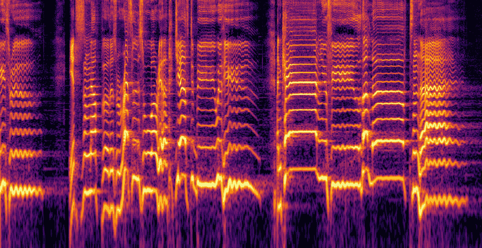
The “Analyst” LLM immediately revealed my most basic misunderstanding. I thought I was feeding a sound model, but that’s not how it works. These models don’t “hear” sound; they “see” it.
Aha! Moment #1: It’s an Image Recognition Problem. The first model in the chain, melspectrogram.onnx, doesn’t process audio waves. Its entire job is to convert a raw 80ms audio chunk into a melspectrogram—a 2D array of numbers that is essentially an image representing the intensity of different frequencies in that sound. The subsequent models are doing pattern recognition on these sound-images, not on the audio itself. This also explained the second part of the puzzle: the models were trained on specifically processed images, which is why this transformation was mandatory:

// This isn't just a normalization; it's part of the "image processing" pipeline
// that the model was trained on. It fails silently without it.
for (let j = 0; j < new_mel_data.length; j++) {
new_mel_data[j] = (new_mel_data[j] / 10.0) + 2.0;
}

The Second Wall: The Audio History Tax

With the formula in place, my test WAV file still failed. The “Analyst” LLM’s breakdown of the Python code’s looping was the key. I realized the pipeline’s second stage needs a history of 76 spectrogram frames to even begin its work. Each 80ms audio chunk only produces 5 frames, meaning the system has to process 16 chunks (1.28 seconds) of audio before it can even think about generating the first feature vector. My test file was too short.

// This logic checks if the audio is long enough and pads it with silence if not.
const minRequiredSamples = 16 * frameSize; // 16 chunks * 1280 samples/chunk = 20480
if (audioData.length < minRequiredSamples) {
const padding = new Float32Array(minRequiredSamples - audioData.length);
const newAudioData = new Float32Array(minRequiredSamples);
newAudioData.set(audioData, 0);
newAudioData.set(padding, audioData.length);
audioData = newAudioData; // Use the new, padded buffer
}

The Third Wall: The Treachery of Optimization

The system came to life, but it was unstable, crashing with a bizarre offset is out of bounds error. This wasn’t a floating-point issue; it was a memory management problem. I discovered that for performance, the ONNX Runtime for web reuses its memory buffers. The variable I was saving wasn’t the data, but a temporary reference to a memory location that was being overwritten.

// AHA Moment: ONNX Runtime reuses its output buffers. We MUST create a *copy*
// of the data instead of just pushing a reference to the buffer.
const new_embedding_data_view = embeddingOut[embeddingModel.outputNames[0]].data;
const stable_copy_of_embedding = new Float32Array(new_embedding_data_view);
embedding_buffer.push(stable_copy_of_embedding); // Push the stable copy, not the temporary view.

The Final Wall: The Purpose of the VAD

The system was finally stable, and I could see the chart spike to 1.0 when I spoke the wake word. But the success sound wouldn’t play reliably. This was due to my most fundamental misconception. I had assumed the VAD’s purpose was to save resources. My thinking was: “VAD is cheap, the wake word model is expensive. So, I should only run the expensive model when the VAD detects speech.”
This is completely wrong.
Aha! Moment #4: The VAD is a Confirmation, Not a Trigger. The wake word pipeline must run continuously to maintain its history buffers. The VAD’s true purpose is to act as a confirmation signal. A detection is only valid if two conditions are met simultaneously: the wake word model reports a high score, AND the VAD confirms that human speech is currently happening. It’s a two-factor authentication system for your voice. This led to the final race condition: the VAD is fast, but the wake word pipeline is slow. The solution was a VAD Hangover—what I call “Redemption Frames”—to keep the detection window open just a little longer.

// These constants define the VAD Hangover logic
const VAD_HANGOVER_FRAMES = 12; // Keep speech active for ~1 second after VAD stops
let vadHangoverCounter = 0;
let isSpeechActive = false;

// Later, the final check uses this managed state:
if (score > 0.5 && isSpeechActive) {
// Detection is valid!
}

The Backend Betrayal: A Final Hurdle

With the core logic finally perfected, I implemented a feature to switch between the WASM, WebGL, and WebGPU backends. WASM and WebGPU worked, but WebGL crashed instantly with the error: `Error: no available backend found. ERR: [wasm] backend not found`.
The issue was that the melspectrogram.onnx model uses specialized audio operators that the WebGL backend in ONNX Runtime simply does not support. My code was trying to force all models onto the selected backend, which is impossible when one is incompatible. The solution was a hybrid backend approach: force the incompatible pre-processing models (melspectrogram and VAD) to run on the universally-supported WASM backend, while allowing the heavy-duty neural network models to run on the user’s selected GPU backend for a performance boost. I’ve left the WebGL option in the demo as a reference for this interesting limitation.

The Final Product

This journey was a powerful lesson in the limitations of “vibe coding” for complex technical problems. While LLMs are incredible for scaffolding, they can’t replace rigorous, first-principles debugging. By pivoting my strategy—using one LLM to deconstruct the source of truth and another to implement that truth—I was able to solve a problem that a single LLM, or even a committee of them, declared impossible. The result is a working, robust web demo that proves this complex audio pipeline can indeed be tamed, running 100% on the client, in the browser, no Python backend required.